1. System architecture modelling and analysis
Welcome to the system architecture modelling and analysis manual. This manual introduces the basic concepts, several applications and our methods and tools for system architecture modelling and analysis.
1.1. Introduction
Engineering design concerns the process of creating solutions in the form of technical systems for problems. The design space is spanned by needs, requirements, and constraints. These can be set by material, technological, economic, legal, environmental and human related considerations.
An important step in the translation of needs, requirements and constraints into technical solutions is the design of the system architecture. The architecture of a system has a significant impact on its performance, e.g., reliability, availability, maintainability, and life cycle costs. Moreover, insight into the system’s architecture is required to estimate the impact of (re)design decisions. That is, the designs of system components are usually dependent on one another. As such, design choices with respect to one component may affect the design of other components. Overlooked dependencies often cause costly and lengthy design iterations.
As systems become increasingly complex the chance on overlooked dependencies increases exponentially. Therefore, engineers need methods to structure, visualize, and analyze needs, requirements, and constraints. This is exactly what Ratio Computer Aided Systems Engineering aims to offer. Our methods and tools aim at supporting engineers to reduce the chance on overlooked dependencies and enable them to develop better systems in less time and at fewer costs.
1.1.1. The engineering design process
In the literature on can find many models of the engineering design process. Figure 1.1 is a schematic representation of the design process which combines the V-model [FM91], spiral model [Boe88] and design phases of Pahl and Beitz [PB07].
Starting at the top left, the requirements (R) at the highest decomposition level are specified. Next, a basic system architecture (A) is defined that denotes the interactions between the conceptual components. Next, a concept (C), i.e. a working-principle and an embodiment (E) are chosen for each component. During detailed design (D) one aims to verify whether the requirements can be fulfilled given the architectural, working-principle and embodiment choices. If so, the first customer validation point is set to check whether the solution satisfies the customer needs thus far. If not, one has to consider other architectures, concepts and embodiments.
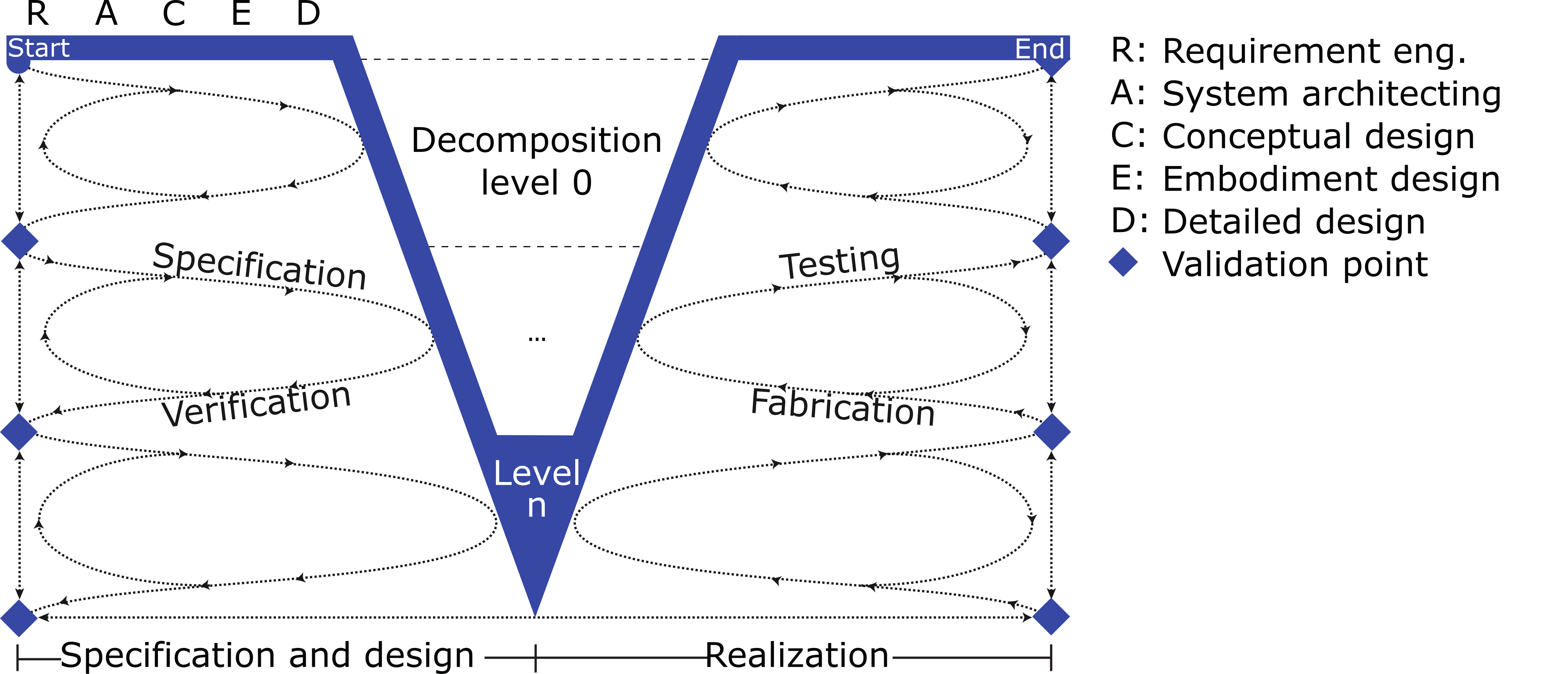
Figure 1.1 Schematic representation of the engineering design process.
Subsequently, one can move to the next decomposition level at which requirements are specified, the architecture is defined, and the concept (working-principles) and embodiment are chosen and verified for all (sub)-components. This process continues until a sufficient level of detail is achieved to start the realization phase (right side of the V). To ensure proper component integration it is essential to have a proper understanding of the system architecture during all phases and at all decomposition levels of the design process. Lack of understanding often leads to costly and lengthy design iterations.
1.1.2. Classical systems engineering
Systems engineering traditionally advocates the use of separate requirement, function, and component trees, as shown in Figure 1.2. Creating dependencies between these trees is done manually. This is a non-trivial, cumbersome and error prone task, which relies heavily on the good-behavior of the modeler to obtain a proper model. Moreover, the neat requirement and function hierarchies often do not exists in real-life. That is, design decisions made during the project often yield new requirements and new functions, which do not fit within the hierarchical structure.
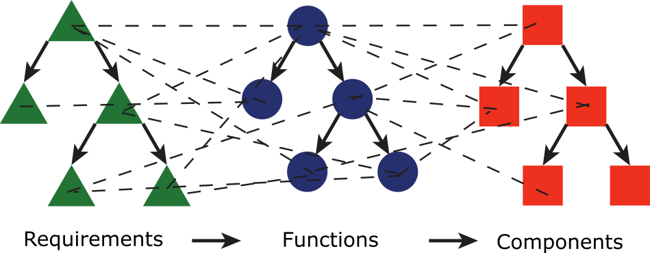
Figure 1.2 Separate requirement, function, and component trees with dependencies between them, as advocated by traditional systems engineering practice.
Finally, the primary goal of the resulting network is to ensure traceability of requirements to functions and physical components. Therefore, it does not represent the system architecture.
Ratio methods and tools build upon the system architecture definition of Ulrich and Eppinger [Ulr95]: “system architecture is the mapping of a system’s functions to the physical components within the system, and to the dependencies between those components”.
1.1.3. Dependency Structure Matrices
In the literature, dependency structure matrix (DSM) methods are commonly used to model, visualize and analyze system architectures in a large variety of industries. The book of Eppinger and Browning [EB12] provides a wide variety of DSM applications in industries and academia alike. A DSM is a square \(N \times N\) matrix in which a non-zero entry at position \((i, j)\) indicates that row element:math:i depends on column element \(j\). A DSM can displays multiple dependency types and strengths at once. Product DSMs are typically used to model dependencies between components.
The two product DSMs on the left of Figure 1.3 display four dependency types between six components. One can highlight the system architecture by re-ordering the matrix using a clustering algorithm. In this case, yielding an integrative (bus) module and two independent modules. This provides opportunities to modularize a system.
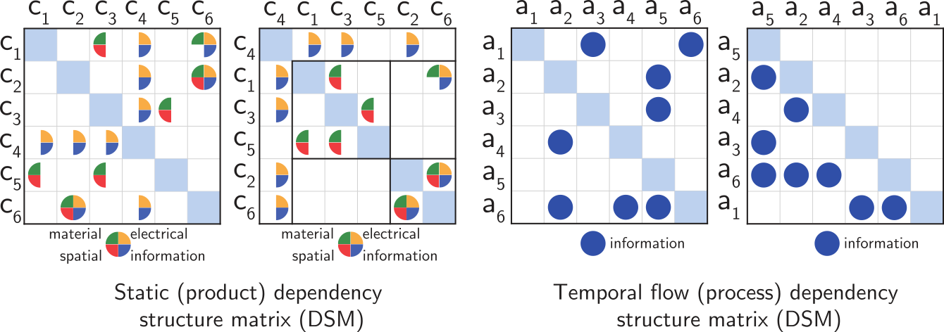
Figure 1.3 Examples of Dependency Structure Matrices.
Process DSMs, as shown on the right of Figure 1.3, are used to model dependencies between functions or (design) parameters. The order of elements along the diagonal of the DSM indicates the sequence in which each element is designed during the process. Sequencing algorithms are used to reduce feedback loops (upper-diagonal marks) which are a source of rework.
1.1.4. The Elephant Specification Language
When systems grow in scale and complexity, it becomes challenging to obtain and maintain an accurate and up-to-date model of the system architecture. Moreover, is is very difficult to ensure the consistency of such a model with the system specifications which are usually written in natural language. To overcome these challenges, Ratio has developed the Elephant Specification Language (ESL) in cooperation with the Eindhoven University of Technology. ESL is specifically developed to enable engineers to write highly structured, multi-level, computer-readable system specifications from which dependencies between requirements, functions, components, variables and combinations thereof can be derived automatically.
In ESL the (functional) requirements are written following a fixed syntax (grammar) within the system decomposition tree, yielding a single structured unambiguous system specification. The ESL compiler performs consistency checks and derives a model of the system architecture. This model can be used to optimize the design and the design process of a system and serves as an interactive visualization of the system specifications.
In the ESL Manual and the ESL Reference Manual ESL is explained in detail. This manual shows how the resulting dependency network can be used to help structure and coordinate your design process and enable you to improve your design. Moreover, it guides you through the various proprietary Python Packages that have been specifically created to process, visualize and analyze ESL specifications in particular and system architecture models in general.
1.2. Overview of applications
This chapter provides a brief overview of system architecture modelling and analysis applications.
1.2.1. Design process organization and coordination
The main reason for creating a system architecture model is to gain better understanding of the system such that one can organize and coordinate the design process more effectively and efficiently. Thereby, improving system quality and reducing engineering time.
Section Dependency Structure Matrices already briefly explained how one can modularize a system by analyzing a product DSM with a clustering algorithm and how one can schedule design activities by analyzing a process DSM with a sequencing algorithm. Furthermore, clustering and sequencing results can be used to determine how to organize design teams or to determine which parts of a system or process can be outsourced.
Figure 1.4 shows a generalized overview of DSM types. In addition to product and process DSM, one can create organization DSM models, multi-domain-matrix (MDM) models, and structure comparison DSM models.
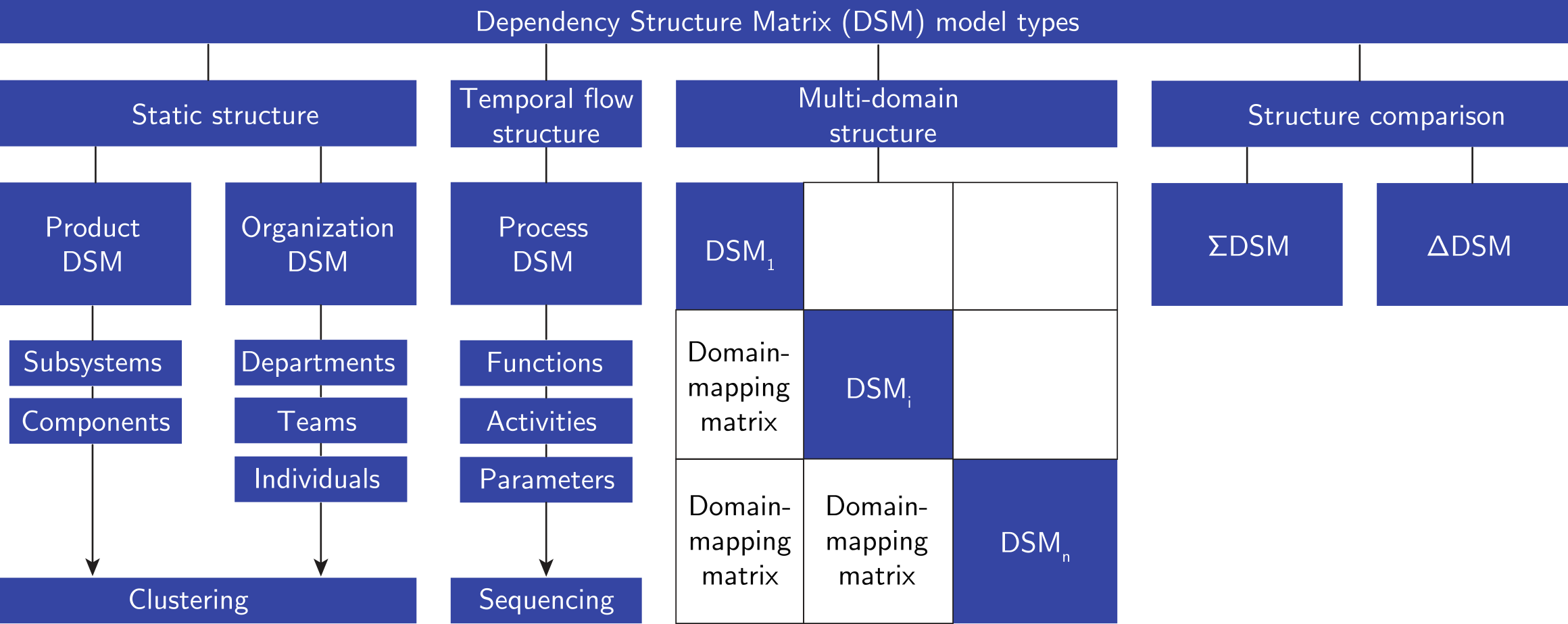
Figure 1.4 Dependency structure matrix types.
An organization DSM shows for example the interactions between people within an organization. In MDM model multiple DSM types are combined into a single figure. An off-diagonal matrix in an MDM is named a domain-mapping-matrix (DMM) and relates elements from one domain to elements in another domain. For example one can combine a product DSM and process DSM into a single figure where the DMM relates components to activities in the design process.
A structure comparison DSM can be used the compare system architectures of multiple systems. An \(\Sigma\)-DSM emphasizes commonalities between system architectures whereas a \(\Delta\)-DSM emphasizes differences.
1.2.2. Modularity Analysis and interface management
One of the most common applications of DSM methods is modularity analysis and interface management. That is, one aims to determine how to best modularize a system such that the different modules can be designed as independently as possible. The interfaces that remain between the different modules need to be carefully managed.
Figure 1.5 shows for example that the reordering of the rows and columns of the DSM one can identify an integrative (bus) module and two component modules.
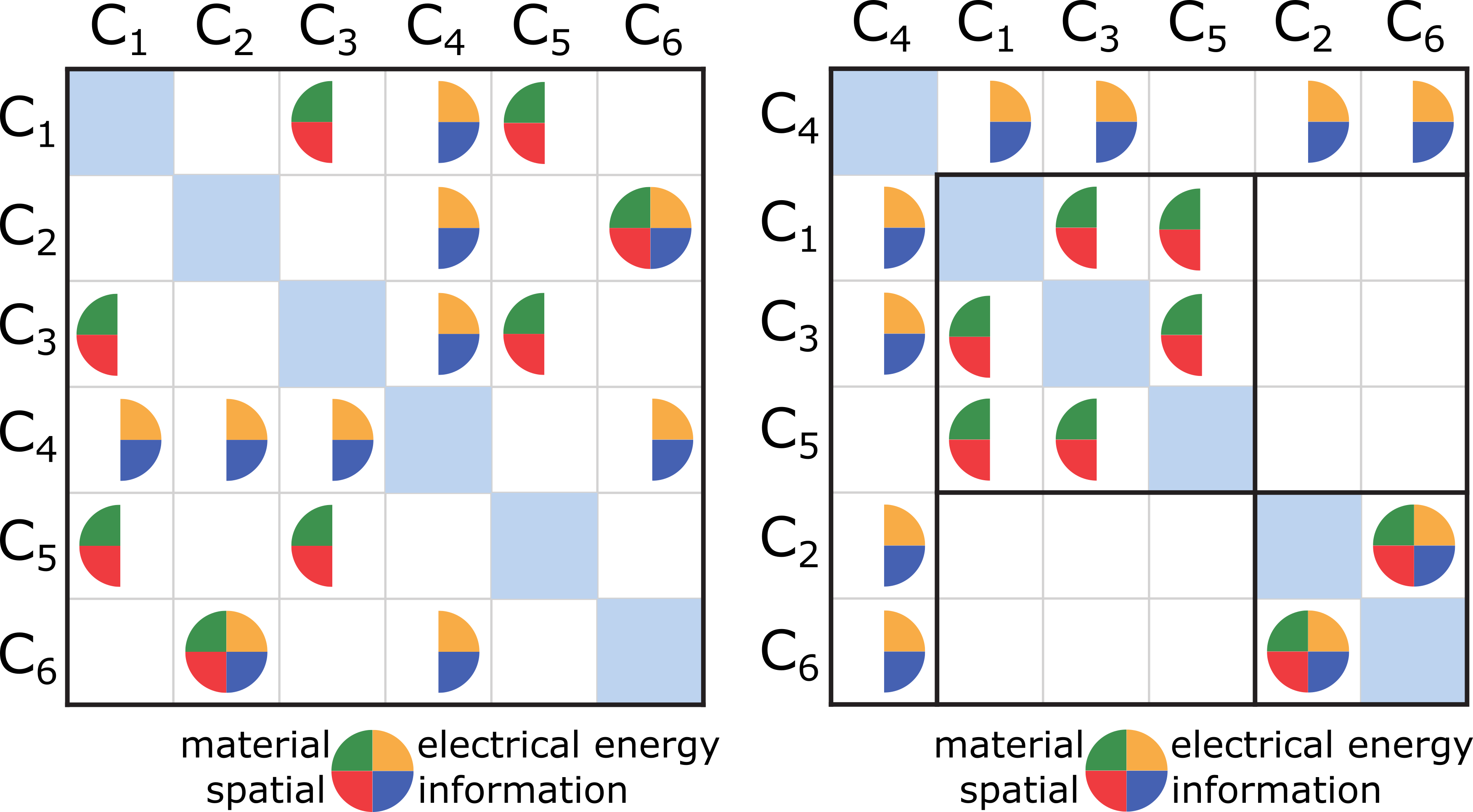
Figure 1.5 Example of a product DSM.
The two component modules can be independently designed, and possibly out-sourced, as long as proper agreements are made concerning the interfaces with bus component c4.
The colours of the dependencies within the matrix indicate which engineering disciplines are required to design the modules and thus need to be part of the design teams.
1.2.3. Risk analysis
A key performance indicator (KPI) is a variable that represents the quality of a system in terms of a certain aspect, e.g., its reliability, availability or cost of ownership. In design processes, resources are often too limited to perform (quantitative) KPI risk analysis for the whole system. A projection dependency structure matrix (P-DSM) enables one to quickly visually identify modules of components critical to various KPI’s. The critical modules are the focus area of subsequent (quantitative) KPI risk analysis.
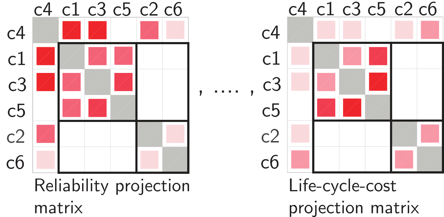
Figure 1.6 Two projection DSMs indicating the areas of interest with respect to reliability and life-cycle-cost, respectively [WERV18b].
For example, the figure on the shows a regular DSM on which reliability (left) and life-cycle-costs (right) impact estimates are projected. These estimates may be a simple low impact (1), medium impact (3) or high impact (9) rating. The brighter the shade of red, the greater the impact of that combination of components on the respective KPI. The reliability P-DSM on the left shows that the combination of components c4, c1 and c3 has the greatest impact on the reliability of the system. The life-cycle cost (LCC) P-DSM shows that the combination of components c1, c3 and c5 has the greatest impact on (LCC). The P-DSMs clearly show the area of interest regarding the respective KPI.
1.2.4. System architecture comparison
During any design process one has to make many design decisions, that may impact the architecture and performance of the system. To visualize the effect of design choices on the system architecture, one can use a comparison dependency structure matrix (C-DSM) as depicted in figure below.
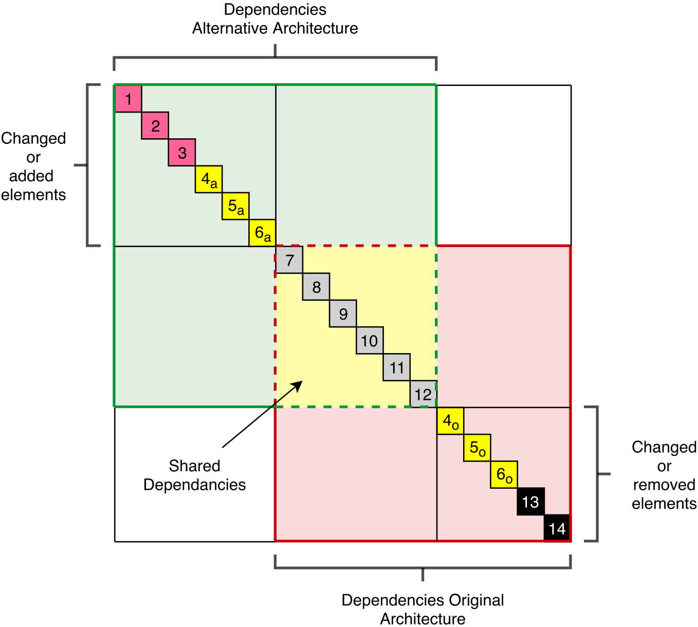
Figure 1.7 Schematic comparison DSM showing the differences between two alternative system architectures [Mee19].
The C-DSM displays two system architectures in a single Figure. The green and red shaded areas contain the elements and dependencies of the two options. Grey elements (7-12) are shared among both architectures. Pink elements (1-3) are only present in the First option. Black elements (13-14) are only present in the second option. Yellow elements (4-6) are present in both options but have different dependencies.
As such, the C-DSM provides a compact overview of the architectural differences between two design alternatives. This overview serves as a ‘discussion figure’ during expert meetings. That is, the system experts can discuss the benefits and down sides of each design alternative by systematically following the figure. This enables them to focus on details while maintaining an overall overview.
1.2.5. Product family design
A major challenge in product family design is to select a realization strategy that balances the external variety offered to the customer with the internal complexity of managing the design, fabrication and maintenance of many different product variants [JSS07].
The figure below shows several realization strategies in relation to the input required for the realization of a product using each strategy. An Engineer-to-Order strategy only requires legislation and customer requirements as input. Subsequently, each product is re-engineered. An Assembly-to-Order strategy requires standard products and customer requirements as input. Subsequently the standard product that best fits the customer requirements is assembled.
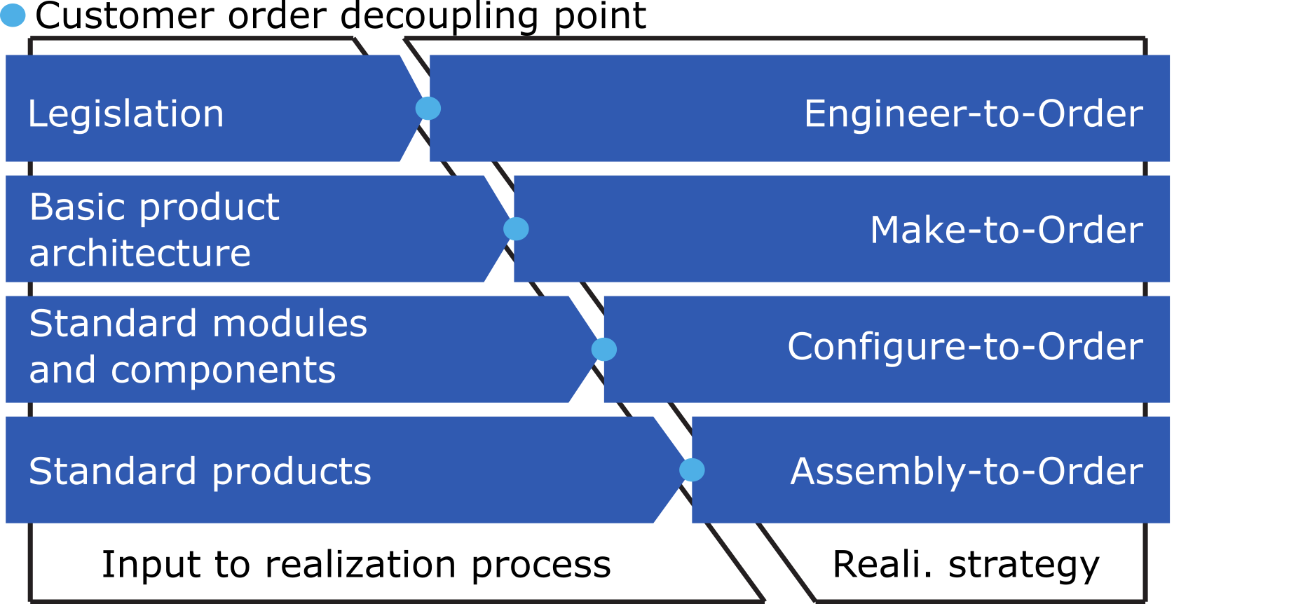
Figure 1.8 Several realization strategies.
Many companies chose a make-to-order or a configure-to-order strategy to offer the customer variety and customization options while minimizing internal complexity. The foundation of such a strategy is a basic product architecture which contains the common core of all product family members. That is, the set of modules of components and their (functional) dependencies that are present in all products. The common core may be extended with optional modules. The basic product architecture should account for these dependencies with optional modules as well to ensure proper and fast component integration once a customer order has been received. Moreover, a basic product architecture enables one to standardize common core and optional modules and the dependencies between them and create a product family platform which further reduces internal complexity.
1.2.6. Product portfolio similarity analysis
The design of a product family requires the creation of a basic product architecture from which all product family members can be derived. By analyzing the similarity of products within an existing product portfolio one can get an indication on which and how many product variants have to be supported by the architecture.
The figure below shows a three step method to find groups of similar products within a diverse product portfolio. Each group represents a variant which must be supported by the basic product architecture.
First, one has to build a binary characteristic mapping matrix M, relating characteristics \(k_i\) to products \(p_i\). Next, one can calculate a product similarity matrix S, indicating how similar two product are based on the selected characteristics. The third step comprises the pruning of S, joining it with M and reordering the matrix with a cluster algorithm. The result provides groups of similar products and shows which characteristics they possess. Here, the products in the first group possess \(k_1\), \(k_2\) and possibly \(k_3\). Products in the second group only possess \(k_3\).
1.2.7. Product portfolio commonality analysis
A product portfolio commonality analysis reveals which modules of components belong to the common core and which are optional within a group of products that form a product family. The commonality analysis starts with building \(n\) binary dependency structure matrices (DSM), one for each variant. Next, one can take the sum of the \(n\) DSMs to obtain a \(\Sigma\)-DSM. The higher the value of a dependency within the \(\Sigma\)-DSM, the more common that combination of components is with the product family. Finally, by clustering the \(\Sigma\)-DSM, one can find modules of components that are common and modules that are optional. For example, in the figure below, five DSMs are summed into a \(\Sigma\)-DSM. Clustering reveals that components c4, c1, c3 and c5 are present in almost all variants, while c2 and c6 are optional. The common components and their dependencies shape the basic product architecture for all variants.
1.3. Tooling
To make life a little bit easier we have created several Python Packages for handling, visualizing and analyzing ESL specifications in particular and graphs in general. You can:
Check out the RaGraph Python Package Docs to create, manipulate, and analyze graphs consisting of nodes and edges that represent system architectures.
Check out the RaESL Python Package Docs to parse and compile ESL files. In the ESL Manual and the ESL Reference Manual ESL is explained in detail.